GrowthMaps.jl

GrowthMaps

GrowthMaps.jl produces gridded population level growth rates from environmental data, and fitted growth and stress models, following the method outlined in Maino et al, "Forecasting the potential distribution of the invasive vegetable leafminer using ‘top-down’ and ‘bottom-up’ models" (in press).

GrowthMaps.jl is a replacement for CLIMEX and similar tools. Different from CLIMEX is that results arrays have units of growth/time. Another useful property of these models is that growth rate layers can be added and combined arbitrarily.

A primary use-case for GrowthMaps layers is in for calculating growth-rates for .

For data input, this package leverages GeoData.jl to import datasets from many different sources. Files are loaded lazily in sequence to minimise memory, using the GeoSeries abstraction, that can hold "SMAP" HDF5 files, NetCDFs, or GeoStacks of tif or other GDAL source files, or simply memory-backed arrays. These data sources can be used interchangeably.

Computations can be run on GPUs, for example with arraytype=CuArray to use CUDA for Nvidia GPUs.

Example

Here we run a single growth model over SMAP data, on a Nvida GPU:

using GrowthMaps, GeoData, HDF5, CUDA, Unitful

# Define a growth model
p = 3e-01
ΔH_A = 3e4cal/mol
ΔH_L = -1e5cal/mol
ΔH_H = 3e5cal/mol
Thalf_L = 2e2K
Thalf_H = 3e2K
T_ref = K(25.0°C)
growthmodel = SchoolfieldIntrinsicGrowth(p, ΔH_A, ΔH_L, Thalf_L, ΔH_H, Thalf_H, T_ref)

# Wrap the model with a data layer with the key
# to retreive the data from, and the Unitful.jl units.
growth = Layer(:surface_temp, K, growthmodel)

Now we will use GeoData.jl to load a series of SMAP files lazily, and GrowthMaps.jl will load them to the GPU just in time for processing:

# Load 1000s of HDF5 files lazily using GeoData.jl
series = SMAPseries("your_SMAP_folder")

# Run the model
output = mapgrowth(growth;
    series=series,
    tspan=DateTime(2016, 1):Month(1):DateTime(2016, 12),
    arraytype=CuArray, # Use an Nvidia GPU for computations
)

# Plot every third month of 2016:
output[Ti(1:3:12)] |> plot

GrowthMaps.jl is fast.

As a rough benchmark, running a model using 3 3800*1600 layers from 3000 SMAP files on a M.2. drive takes under 7 minutes on a desktop with a good GPU, like a GeForce 1080. The computation time is trivial, running ten similar models takes essentially the same time as running one model. On a CPU, model run-time becomes more of a factor, but is still fast for a single model.

See the Examples section in the documentation to get started. You can also work through the example.jmd in atom (with the language-weave plugin) or the notebook.

Live Interfaces

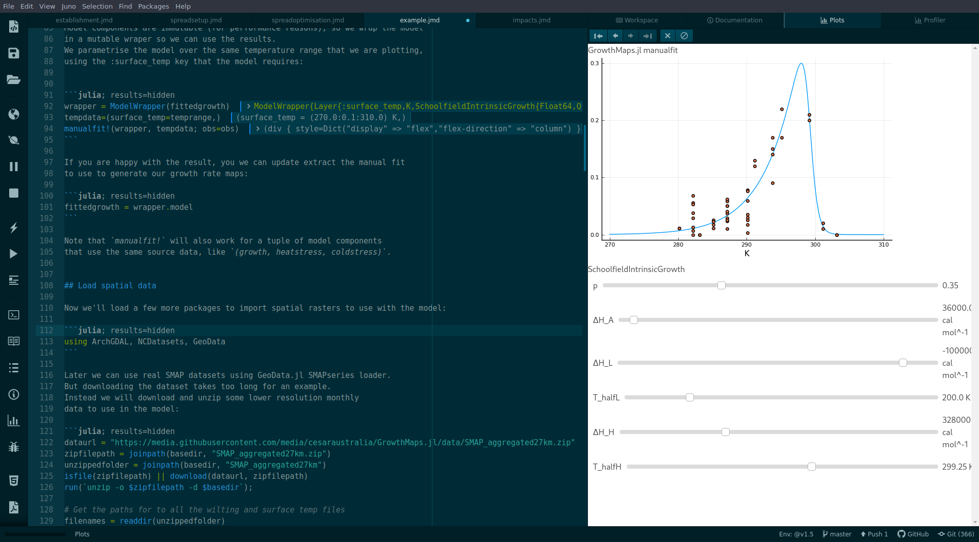
GrowthMaps provides interfaces for manually fitting models where automated fits are not appropriate.

Model curves can be fitted to an AbstractRange of input data using manualfit:

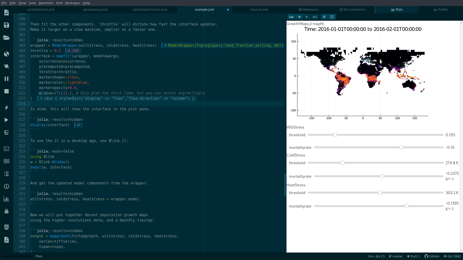
Observations can be fitted to a map. Aggregated maps GeoSeries can be used to fit models in real-time. See the examples for details.

The intrinsic rate of population growth is the exponential growth rate of a population when growth is not limited by density dependent factors.

More formally, if the change in population size $N$ with time $t$ is expressed as $\frac{dN}{dt} = rN$, then $r$ is the intrinsic population growth rate (individuals per day per individual) which can be decomposed into per capita reproduction and mortality rate. The intrinsic growth rate parameter $r$ depends strongly on temperature, with population growth inhibited at low and high temperatures (Haghani et al. 2006).

This can be described using a variety of non-linear functions, see SchoolfieldIntrinsicGrowth for an implementation.

Layer{K,U}(model::RateModel)
Layer(key::Symbol, model::RateModel)
Layer(key::Symbol, u::Union{Units,Quantity}, model::RateModel)

Layers connect a model to a data source, providing the key to look up the layer in a GeoData.jl GeoStack, and specifying the scientific units of the layer, if it has units. Using units adds an extra degree of safety to your calculation, and allows for using data in different units with the same models.

LowerStress(key::Symbol, threshold, mortalityrate)

A StressModel where stress occurs below a threshold at a specified mortalityrate for some environmental layer key.

Independent variables must be in the same units as

Passed to an optimiser to facilitate fitting any RateModel, without boilerplate or methods rewrites.

Update the model with passed in params, and run [rate] over the independent variables.

A RateModel conatains the parameters to calculate the contribution of a growth or stress factor to the overall population growth rate.

A rate method corresponding to the model type must be defined specifying the formulation, and optionally a condition method to e.g. ignore data below thresholds.

SchoolfieldIntrinsicGrowth(p, ΔHA, ΔHL, ΔHH, ThalfL, ThalfH, Tref, R)

A GrowthModel where the temperature response of positive growth rate is modelled following Schoolfield et al. 1981, "Non-linear regression of biological temperature-dependent rate models base on absolute reaction-rate theory".

The value of the specified data layer must be in Kelvin.

Arguments

• p::P: growth rate at reference temperature T_ref
• ΔH_A: enthalpy of activation of the reaction that is catalyzed by the enzyme, in cal/mol or J/mol.
• ΔH_L: change in enthalpy associated with low temperature inactivation of the enzyme.
• ΔH_H: change in enthalpy associated with high temperature inactivation of the enzyme.
• T_halfL: temperature (Unitful K) at which the enzyme is 1/2 active and 1/2 low temperature inactive.
• T_halfH: temperature (Unitful K) at which the enzyme is 1/2 active and 1/2 high temperature inactive.
• T_ref: Reference temperature in kelvin.

This can be parameterised from empirical data, (see Zhang et al. 2000; Haghani et al. 2006; Chien and Chang 2007) and non-linear least squares regression.

Extreme stressor mortality can be assumed to occur once an environmental variable $s$ exceeds some threshold (e.g. critical thermal maximum), beyond which the mortality rate scales approximately linearly with the depth of the stressor (Enriquez and Colinet 2017).

Stressor induced mortality is incorporated in growth rates by quantifying the threshold parameter $s_c$ beyond which stress associated mortality commences, and the mortalityrate parameter $m_s$ which reflects the per-capita mortality per stress unit, per time (e.g. degrees beyond the stress threshold per day).

When stressors are combined in a model, the mortality rate for each stressor $s$ is incorporated as $\frac{dN}{dt}=(r_p-r_n)N$ where $r_n = \sum{s}f(s, c_s)m_s$ and $f(s, c_s)$ is a function that provides the positive units by which s exceeds $s_c$.

This relies on the simplifying assumption that different stressors contribute additively to mortality rate, but conveniently allows the mortality response of stressors to be partitioned and calculated separately to the intrinsic growth rate, which aids parameterisation and modularity. More complicated stress responses are more likely to capture reality more completely, but the availability of data on detailed mortality responses to climatic stressors is often lacking.

Upper and lower stresses may be in relation to any environmental variable, specied with the key parameter, that will use the data at that key in GeoStack for the current timestep.

UpperStress(key::Symbol, threshold, mortalityrate)

A StressModel where stress occurs above a threshold at the specified mortalityrate, for some environmental layer key.

condition(m, x)

Subseting the data before applying the rate method, given the model m and the environmental variable of value x. Returns a boolean. If not defined, defaults to true for all values.

fit!(model::ModelWrapper, obs::AbstractArray)

Run fit on the contained model, and write the updated model to the mutable modelwrapper.

fit(model, obs::AbstractArray)

Fit a model to data with least squares regression, using curve_fit from LsqFit.jl. The passed in model should be initialised with sensible defaults, these will be used as the initial parameters for the optimization.

Any (nested) Real fields on the struct are flattened to a parameter vector using Flatten.jl. Fields can be marked to ignore using the @flattenable macro from FieldMetadata.jl.

Arguments

• model: Any constructed RateModel or a Tuple of RateModel.
• obs: Vector of observations, such as length 2 Tuples of Real. Leave units off.

Returns

An updated model with fitted parameters.

manualfit!(wrapper::ModelWrapper, ranges::Array; obs=[],  kwargs...) =

Returns the wrapper with the fitted model.

• obs: A Vector of (val, rate) tuples/vectors
• data:

Example

p = 3e-01
ΔH_A = 3e4cal/mol
ΔH_L = -1e5cal/mol
ΔH_H = 3e5cal/mol
Thalf_L = 2e2K
Thalf_H = 3e2K
T_ref = K(25.0°C)
growthmodel = SchoolfieldIntrinsicGrowth(p, ΔH_A, ΔH_L, Thalf_L, ΔH_H, Thalf_H, T_ref)
model = ModelWrapper(Layer(:surface_temp, K, growthmodel))
obs = []

tempdata=(surface_temp=(270.0:0.1:310.0)K,)
manualfit!(model, tempdata; obs=obs)

To use the interface in a desktop app, use Blink.jl:

julia; eval=false using Blink w = Blink.Window() body!(w, interface) ```

mapfit!(wrapper::ModelWrapper, modelkwargs; occurrence=[], precomputed=nothing, kwargs...)

Fit a model to the map.

Example

wrapper = ModelWrapper(wiltstress, coldstress, heatstress)
throttle = 0.2
interface = mapfit!(wrapper, modelkwargs;
    occurrence=occurrence,
    precomputed=precomputed,
    throttle=throttle,
    markershape=:cross,
    markercolor=:lightblue,
    markeropacity=0.4
)
display(interface)

To use the interface in a desktop app, use Blink.jl:

using Blink
w = Blink.Window()
body!(w, interface)

mapgrowth(models; series::AbstractGeoSeries, tspan::AbstractRange, arraytype=Array) => GeoArray

Combine growth rates and stressors for all layers, in all files in each series falling in each period of tspan.

Arguments

• models: a ModelWrapper, a Tuple or splat of Layer components, or a NamedTuple holding multiple Tuple/ModelWrapper models.

Keyword Arguments

• series: any AbstractGeoSeries from GeoData.jl
• tspan: AbstractRange for the timespan to run the layers for. This will be the index oof the output Ti dimension.
• arraytype: An array constructor to apply to data once it's loaded from disk. The main use case for this is a GPUArray such as CuArray which will result in all computations happening on the GPU, if you have one.

Using multiple models in a NamedTuple can be an order of magnitude faster than running models separately – especially when arraytype=CuArray or similar. In this configuration, all data required by all layers in all models will be loaded from disk only once and copied to the GPU only once. This is useful for doing all kinds of sensitivity analysis and model comparison.

Returns

A GeoArray or NamedTuple of GeoArray, with the same dimensions as the passed-in stack layers, and an additional Ti (time) dimension matching tspan.

rate(m, x)

Calculates the rate modifyer for a single cell. Must be defined for all models.

m is the object containing the model parameters, and x is the value at a particular location for of an environmental variable specified by the models key() method, using corresponding to its key field.