DynamicGrids
DynamicGrids — Module![]()
![]()
![]()

![]()
DynamicGrids is a generalised framework for building high-performance grid-based spatial simulations, including cellular automata, but also allowing a wider range of behaviours like random jumps and interactions between multiple grids. It is extended by Dispersal.jl for modelling organism dispersal processes.
DynamicGridsGtk.jl provides a simple live interface, while DynamicGridsInteract.jl also has live control over model parameters while the simulation runs: real-time visual feedback for manual parametrisation and model exploration.
DynamicGrids can run rules on single CPUs, threaded CPUs, and on CUDA GPUs. Simulation run-time is usually measured in fractions of a second.
A dispersal simulation with quarantine interactions, using Dispersal.jl, custom rules and the GtkOuput from DynamicGridsGtk. Note that this is indicative of the real-time frame-rate on a laptop.
A DynamicGrids.jl simulation is run with a script like this one running the included game of life model Life():
using DynamicGrids, Crayons

init = rand(Bool, 150, 200)
output = REPLOutput(init; tspan=1:200, fps=30, color=Crayon(foreground=:red, background=:black, bold=true))
sim!(output, Life())

# Or define it from scratch (yes this is actually the whole implementation!)
life = Neighbors(Moore(1)) do data, hood, state, I
    born_survive = (false, false, false, true, false, false, false, false, false),
                   (false, false, true, true,  false, false, false, false, false)
    born_survive[state + 1][sum(hood) + 1]
end
sim!(output, life)
A game of life simulation being displayed directly in a terminal.
Concepts
The framework is highly customisable, but there are some central ideas that define how a simulation works: grids, rules, and outputs.
Grids
Simulations run over one or many grids, derived from init of a single AbstractArray or a NamedTuple of multiple AbstractArray. Grids (GridData types) are, however not a single array but both source and destination arrays, to maintain independence between cell reads and writes where required. These may be padded or otherwise altered for specific performance optimisations. However, broadcasted getindex operations are guaranteed to work on them as if the grid is a regular array. This may be useful running simulations manually with step!.
Grid contents
Often grids contain simple values of some kind of Number, but other types are possible, such as SArray, FieldVector or other custom structs. Grids are updated by Rules that are run for every cell, at every timestep.
NOTE: Grids of mutable objects (e.g Array or any mutable struct have undefined behaviour. DynamicGrids.jl does not deepcopy grids between frames as it is expensive, so successive frames will contain the same objects. Mutable objects will not work at all on GPUs, and are relatively slow on CPUs. Instead, use regular immutable structs and StaticArrays.jl if you need arrays. Update them using @set from Setfield.jl or Accessors.jl, and generally use functional programming approaches over object-oriented ones.
Init
The init grid/s contain whatever initialisation data is required to start a simulation: the array type, size and element type, as well as providing the initial conditions:
init = rand(Float32, 100, 100)An init grid can be attached to an Output:
output = ArrayOutput(init; tspan=1:100)or passed in to sim!, where it will take preference over the init attached to the Output, but must be the same type and size:
sim!(output, ruleset; init=init)For multiple grids, init is a NamedTuple of equal-sized arrays matching the names used in each Ruleset :
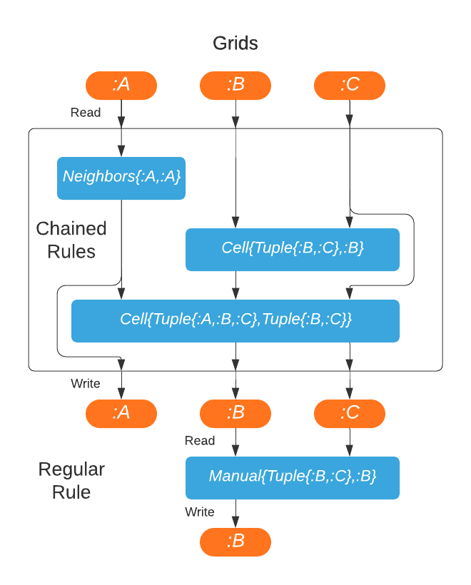
init = (predator=rand(100, 100), prey=(rand(100, 100))Handling and passing of the correct grids to a Rule is automated by DynamicGrids.jl, as a no-cost abstraction. Rules specify which grids they require in what order using the first two (R and W) type parameters.
Dimensional or spatial init grids from DimensionalData.jl or GeoData.jl will propagate through the model to return output with explicit dimensions. This will plot correctly as a map using Plots.jl, to which shape files and observation points can be easily added.
Non-Number Grids
Grids containing custom and non-Number types are possible, with some caveats. They must define Base.zero for their element type, and should be a bitstype for performance. Tuple does not define zero. Array is not a bitstype, and does not define zero. SArray from StaticArrays.jl is both, and can be used as the contents of a grid. Custom structs that defne zero should also work.
However, for any multi-values grid element type, you will need to define a method of DynamicGrids.to_rgb that returns an ARGB32 for them to work in ImageOutputs, and isless for the REPLoutput to work. A definition for multiplication by a scalar Real and addition are required to use Convolution kernels.
Rules
Rules hold the parameters for running a simulation, and are applied in applyrule method that is called for each of the active cells in the grid. Rules come in a number of flavours (outlined in the docs). This allows using specialised methods for different types of rules, ecoding assumtions about their behaviours that can greatly improve performance through more efficient use of caches and parallelisation. Rules can be collected in a Ruleset, with some additional arguments to control the simulation:
ruleset = Ruleset(Life(2, 3); opt=SparseOpt(), proc=CuGPU())Multiple rules can be combined in a Ruleset or simply passed to sim! directly. Each rule will be run for the whole grid, in sequence, using appropriate optimisations depending on the parent types of each rule:
ruleset = Ruleset(rule1, rule2; timestep=Day(1), opt=SparseOpt(), proc=ThreadedCPU())Output
Outputs are ways of storing or viewing a simulation. They can be used interchangeably depending on your needs: ArrayOutput is a simple storage structure for high performance-simulations. As with most outputs, it is initialised with the init array, but in this case it also requires the number of simulation frames to preallocate before the simulation runs.
output = ArrayOutput(init; tspan=1:10)The REPLOutput shown above is a GraphicOutput that can be useful for checking a simulation when working in a terminal or over ssh:
output = REPLOutput(init; tspan=1:100)ImageOutput is the most complex class of outputs, allowing full color visual simulations using ColorSchemes.jl. It can also display multiple grids using color composites or layouts, as shown above in the quarantine simulation.
DynamicGridsInteract.jl provides simulation interfaces for use in Juno, Jupyter, web pages or electron apps, with live interactive control over parameters, using ModelParameters.jl. DynamicGridsGtk.jl is a simple graphical output for Gtk. These packages are kept separate to avoid dependencies when being used in non-graphical simulations.
Outputs are also easy to write, and high performance applications may benefit from writing a custom output to reduce memory use, or using TransformedOuput. Performance of DynamicGrids.jl is dominated by cache interactions, so reducing memory use has positive effects.
Example: Forest Fire
This example implements the classic stochastic forest fire model in a few different ways, and benchmarks them. Note you will need ImageMagick.jl installed for .gif output to work.
First we will define a Forest Fire algorithm that sets the current cell to burning, if a neighbor is burning. Dead cells can come back to life, and living cells can spontaneously catch fire:
using DynamicGrids, ColorSchemes, Colors, BenchmarkTools

const DEAD, ALIVE, BURNING = 1, 2, 3

neighbors_rule = let prob_combustion=0.0001, prob_regrowth=0.01
    Neighbors(Moore(1)) do data, neighborhood, cell, I
        if cell == ALIVE
            if BURNING in neighborhood
                BURNING
            else
                rand() <= prob_combustion ? BURNING : ALIVE
            end
        elseif cell == BURNING
            DEAD
        else
            rand() <= prob_regrowth ? ALIVE : DEAD
        end
    end
end

# Set up the init array and output (using a Gtk window)
init = fill(ALIVE, 400, 400)
output = GifOutput(init;
    filename="forestfire.gif",
    tspan=1:200,
    fps=25,
    minval=DEAD, maxval=BURNING,
    scheme=ColorSchemes.rainbow,
    zerocolor=RGB24(0.0)
)

# Run the simulation, which will save a gif when it completes
sim!(output, neighbors_rule)
Timing the simulation for 200 steps, the performance is quite good. This particular CPU has six cores, and we get a 5.25x speedup by using all of them, which indicates good scaling:
bench_output = ResultOutput(init; tspan=1:200)

julia>
@btime sim!($bench_output, $neighbors_rule);
  477.183 ms (903 allocations: 2.57 MiB)

julia> @btime sim!($bench_output, $neighbors_rule; proc=ThreadedCPU());
  91.321 ms (15188 allocations: 4.07 MiB)
We can also invert the algorithm, setting cells in the neighborhood to burning if the current cell is burning, by using the SetNeighbors rule:
setneighbors_rule = let prob_combustion=0.0001, prob_regrowth=0.01
    SetNeighbors(Moore(1)) do data, neighborhood, cell, I
        if cell == DEAD
            if rand() <= prob_regrowth
                data[I...] = ALIVE
            end
        elseif cell == BURNING
            for pos in positions(neighborhood, I)
                if data[pos...] == ALIVE
                    data[pos...] = BURNING
                end
            end
            data[I...] = DEAD
        elseif cell == ALIVE
            if rand() <= prob_combustion
                data[I...] = BURNING
            end
        end
    end
end
Note: we are not using add!, instead we just set the grid value directly. This usually risks errors if multiple cells set different values. Here they only ever set a currently living cell to burning in the next timestep. It doesn't matter if this happens multiple times, the result is the same.
And in this case (a fairly sparse simulation), this rule is faster:
julia> @btime sim!($bench_output, $setneighbors_rule);
  261.969 ms (903 allocations: 2.57 MiB)

julia> @btime sim!($bench_output, $setneighbors_rule; proc=ThreadedCPU());
  65.489 ms (7154 allocations: 3.17 MiB)
But the scaling is not quite as good, at 3.9x for 6 cores. The first method may be better on a machine with a lot of cores.
Last, we slightly rewrite these rules for GPU, as rand was not available within a GPU kernel. It is now, but it turns out that this method is faster! and interesting to demonstrate using multiple grids and SetGrid.
This way we call CUDA.rand! on the entire parent array of the :rand grid, using a SetGrid rule:
using CUDAKernels, CUDA

randomiser = SetGrid{Tuple{},:rand}() do randgrid
    CUDA.rand!(parent(randgrid))
end
Now we define a Neighbors version for GPU, using the :rand grid values instead of rand():
neighbors_gpu = let prob_combustion=0.0001, prob_regrowth=0.01
    Neighbors{Tuple{:ff,:rand},:ff}(Moore(1)) do data, neighborhood, (cell, rand), I
        if cell == ALIVE
            if BURNING in neighborhood
                BURNING
            else
                rand <= prob_combustion ? BURNING : ALIVE
            end
        elseif cell == BURNING
            DEAD
        else
            rand <= prob_regrowth ? ALIVE : DEAD
        end
    end
end
And a SetNeighbors version for GPU:
setneighbors_gpu = let prob_combustion=0.0001, prob_regrowth=0.01
    SetNeighbors{Tuple{:ff,:rand},:ff}(Moore(1)) do data, neighborhood, (cell, rand), I
        if cell == DEAD
            if rand <= prob_regrowth
                data[:ff][I...] = ALIVE
            end
        elseif cell == BURNING
            for pos in positions(neighborhood, I)
                if data[:ff][pos...] == ALIVE
                    data[:ff][pos...] = BURNING
                end
            end
            data[:ff][I...] = DEAD
        elseif cell == ALIVE
            if rand <= prob_combustion
                data[:ff][I...] = BURNING
            end
        end
    end
end
Now benchmark both version on a GTX 1080 GPU. Despite the overhead of reading and writing two grids, this turns out to be even faster again:
bench_output_rand = ResultOutput((ff=init, rand=zeros(size(init))); tspan=1:200)

julia> @btime sim!($bench_output_rand, $randomiser, $neighbors_gpu; proc=CuGPU());
  30.621 ms (186284 allocations: 17.19 MiB)

julia> @btime sim!($bench_output_rand, $randomiser, $setneighbors_gpu; proc=CuGPU());
  22.685 ms (147339 allocations: 15.61 MiB)
That is, we are running the rule at a rate of 1.4 billion times per second. These timings could be improved (maybe 10-20%) by using grids of Int32 or Int16 to use less memory and cache. But we will stop here.
Running simulations
DynamicGrids.sim! — Functionsim!(output, rules::Rule...; kw...)
sim!(output, rules::Tuple{<:Rule,Vararg}; kw...)
sim!(output, [ruleset::Ruleset=ruleset(output)]; kw...)Runs the simulation rules over the output tspan, writing the destination array to output for each time-step.
Arguments
output: AnOutputto store grids or display them on the screen.ruleset: ARulesetcontaining one or moreRules. If the output has aRulesetattached, it will be used.
Keywords
Theses are the taken from the output argument by default:
init: optional array or NamedTuple of arrays.mask: aBoolarray matching the init array size.falsecells do not run.aux: aNamedTupleof auxilary data to be used by rules.tspan: a tuple holding the start and end of the timespan the simulaiton will run for.fps: the frames per second to display. Will be taken from the output if not passed in.
Theses are the taken from the ruleset argument by default:
proc: aProcessorto specificy the hardware to run simulations on, likeSingleCPU,ThreadedCPUorCuGPUwhen KernelAbstractions.jl and a CUDA gpu is available.opt: aPerformanceOptto specificy optimisations likeSparseOptorNoOpt. Defaults toNoOpt().boundary: what to do with boundary of grid edges. Options areRemoveorWrap, defaulting toRemove().cellsize: the size of cells, which may be accessed by rules.timestep: fixed timestep where this is required for some rules. eg.Month(1)or1u"s".
Other:
simdata: aSimDataobject. Keeping it between simulations can reduce memory allocation a little, when that is important.
DynamicGrids.resume! — Functionresume!(output::GraphicOutput, ruleset::Ruleset=ruleset(output); tstop, kw...)Restart the simulation from where you stopped last time. For arguments see sim!. The keyword arg tstop can be used to extend the length of the simulation.
Arguments
output: AnOutputto store grids or display them on the screen.ruleset: ARulesetcontaining one ore moreRules. These will each be run in sequence.
Keywords (optional)
tstop: the new stop time for the simulation. Taken from the output length by default.fps: the frames per second to display. Taken from the output by default.simdata: aSimDataobject. Keeping it between simulations can improve performance when that is important
DynamicGrids.step! — Functionstep!(sd::AbstractSimData)Allows stepping a simulation one frame at a time, for a more manual approach to simulation that sim!. This may be useful if other processes need to be run between steps, or the simulation is of variable length. step! also removes the use of Outputs, meaning storing of grid data must be handled manually, if that is required. Of course, an output can also be updated manually, using:
DynmicGrids.storeframe!(output, simdata)Instead of an Output, the internal SimData objects are used directly, and can be defined using a Extent object and a Ruleset.
Example
using DynmicGrids, Plots
ruleset = Ruleset(Life(); proc=ThreadedCPU())
extent = Extent(; init=(a=A, b=B), aux=aux, tspan=tspan)
simdata = SimData(extent, ruleset)

# Run a single step, which returns an updated `SimData` object
simdata = step!(simdata)
# Get a view of the grid without padding
grid = DynmicGrids.gridview(simdata[:a])
heatmap(grid)
This example returns a GridData object for the :a grid, which is <: AbstractAray.
Rulesets
DynamicGrids.AbstractRuleset — TypeAbstractRuleset <: ModelParameters.AbstractModelAbstract supertype for Ruleset objects and variants.
DynamicGrids.Ruleset — TypeRulseset <: AbstractRuleset
Ruleset(rules...; kw...)
Ruleset(rules, settings)A container for holding a sequence of Rules and simulation details like boundary handing and optimisation. Rules will be run in the order they are passed, ie. Ruleset(rule1, rule2, rule3).
Keywords
proc: aProcessorto specificy the hardware to run simulations on, likeSingleCPU,ThreadedCPUorCuGPUwhen KernelAbstractions.jl and a CUDA gpu is available.opt: aPerformanceOptto specificy optimisations likeSparseOpt. Defaults toNoOpt.boundary: what to do with boundary of grid edges. Options areRemove()orWrap(), defaulting toRemove.cellsize: size of cells.timestep: fixed timestep where this is required for some rules. eg.Month(1)or1u"s".
Options/Flags
Boundary conditions
DynamicGrids.BoundaryCondition — TypeBoundaryConditionAbstract supertype for flags that specify the boundary conditions used in the simulation, used in inbounds and to update NeighborhoodRule grid padding. These determine what happens when a neighborhood or jump extends outside of the grid.
DynamicGrids.Wrap — TypeWrap <: BoundaryCondition
Wrap()BoundaryCondition flag to wrap cordinates that boundary boundaries back to the opposite side of the grid.
Specifiy with:
ruleset = Ruleset(rule; boundary=Wrap())
# or
output = sim!(output, rule; boundary=Wrap())DynamicGrids.Remove — TypeRemove <: BoundaryCondition
Remove()BoundaryCondition flag that specifies to assign padval to cells that overflow grid boundaries. padval defaults to zero(eltype(grid)) but can be assigned as a keyword argument to an Output.
Specifiy with:
ruleset = Ruleset(rule; boundary=Remove())
# or
output = sim!(output, rule; boundary=Remove())Hardware selection
DynamicGrids.Processor — TypeProcessorAbstract supertype for selecting a hardware processor, such as ia CPU or GPU.
DynamicGrids.CPU — TypeCPU <: ProcessorAbstract supertype for CPU processors.
DynamicGrids.SingleCPU — TypeSingleCPU <: CPU
SingleCPU()Processor flag that specifies to use a single thread on a single CPU.
Specifiy with:
ruleset = Ruleset(rule; proc=SingleCPU())
# or
output = sim!(output, rule; proc=SingleCPU())DynamicGrids.ThreadedCPU — TypeThreadedCPU <: CPU
ThreadedCPU()Processor flag that specifies to use a Threads.nthreads() CPUs.
Specifiy with:
ruleset = Ruleset(rule; proc=ThreadedCPU())
# or
output = sim!(output, rule; proc=ThreadedCPU())DynamicGrids.GPU — TypeGPU <: ProcessorAbstract supertype for GPU processors.
DynamicGrids.CuGPU — TypeCuGPU <: GPU
CuGPU()
CuGPU{threads_per_block}()ruleset = Ruleset(rule; proc=CuGPU())
# or
output = sim!(output, rule; proc=CuGPU())DynamicGrids.CPUGPU — TypeCPUGPU <: GPU
CPUGPU()Uses the CUDA GPU code on CPU using KernelAbstractions, to test it.
Performance optimisation
DynamicGrids.PerformanceOpt — TypePerformanceOptAbstract supertype for performance optimisation flags.
DynamicGrids.NoOpt — TypeNoOpt <: PerformanceOpt
NoOpt()Flag to run a simulation without performance optimisations besides basic high performance programming. Still fast, but not intelligent about the work that it does: all cells are run for all rules.
NoOpt is the default opt method.
DynamicGrids.SparseOpt — TypeSparseOpt <: PerformanceOpt
SparseOpt()An optimisation flag that ignores all padding valuesin the grid, by default zeros.
For low-density simulations performance may improve by orders of magnitude, as only used cells are run.
Specifiy with:
ruleset = Ruleset(rule; opt=SparseOpt())
# or
output = sim!(output, rule; opt=SparseOpt())
SparseOpt is best demonstrated with this simulation, where the grey areas do not run except where the neighborhood partially hangs over an area that is not grey:
Rules
DynamicGrids.Rule — TypeRuleA Rule object contains the information required to apply an applyrule method to every cell of every timestep of a simulation.
The applyrule method follows the form:
@inline applyrule(data::AbstractSimData, rule::MyRule, state, I::Tuple{Int,Int}) = ...Where I is the cell index, and state is a single value, or a NamedTuple if multiple grids are requested. the AbstractSimData object can be used to access current timestep and other simulation data and metadata.
Rules can be updated from the original rule before each timestep, in modifyrule. Here a paremeter depends on the sum of a grid:
using DynamicGrids, Setfield
struct MySummedRule{R,W,T} <: CellRule{R,W}
    gridsum::T
end
function modifyrule(rule::MySummedRule{R,W}, data::AbstractSimData) where {R,W}
    Setfield.@set rule.gridsum = sum(data[R])
end

# output
modifyrule (generic function with 1 method)
Rules can also be run in sequence, as a Tuple or in a Rulesets.
DynamicGrids guarantees that:
modifyruleis run once for every rule for every timestep. The result is passed toapplyrule, but not retained after that.applyruleis run once for every rule, for every cell, for every timestep, unless an optimisation likeSparseOptis used to skip empty cells.- the output of running a rule for any cell does not affect the input of the same rule running anywhere else in the grid.
- rules later in the sequence are passed grid state updated by the earlier rules.
- masked areas, and wrapped or removed
boundaryregions are updated between rules when they have changed.
Multiple grids
The keys of the init NamedTuple will be match the grid keys used in R and W for each rule, which is a type like Tuple{:key1,:key1}. Note that the names are user-specified, and should never be fixed by a Rule.
Read grid names are retrieved from the type here as R1 and R2, while write grids are W1 and W2.
using DynamicGrids
struct MyMultiSetRule{R,W} <: SetCellRule{R,W} end
function applyrule(
    data::AbstractSimData, rule::MyMultiSetRule{Tuple{R1,R2},Tuple{W1,W2}}, (r1, r2), I
) where {R1,R2,W1,W2}
    add!(data[W1], 1, I)
    add!(data[W2], 1, I)
end

# output
applyrule (generic function with 1 method)
The return value of an applyrule is written to the current cell in the specified W write grid/s. Rules writing to multiple grids simply return a Tuple in the order specified by the W type params.
Rule Performance
Rules may run many millions of times during a simulation. They need to be fast. Some basic guidlines for writing rules are:
- Never allocate memory in a
Ruleif you can help it. - Type stability is essential.
isinferredis useful to check if your rule is type-stable. - Using the
@inlinemacro onapplyrulecan help force inlining your code into the simulation. - Reading and writing from multiple grids is expensive due to additional load on fast cahce memory. Try to limit the number of grids you use.
- Use a graphical profiler, like ProfileView.jl, to check your rules overall performance when run with
sim!.
DynamicGrids.SetRule — TypeSetRule <: RuleAbstract supertype for rules that manually write to the grid in some way.
These must define methods of applyrule!.
CellRule
DynamicGrids.CellRule — TypeCellrule <: RuleA Rule that only writes and uses a state from single cell of the read grids, and has its return value written back to the same cell(s).
This limitation can be useful for performance optimisation, such as wrapping rules in Chain so that no writes occur between rules.
CellRule is defined with :
using DynamicGrids
struct MyCellRule{R,W} <: CellRule{R,W} end
# output
And applied as:
function applyrule(data, rule::MyCellRule, state, I)
    state * 2
end
# output
applyrule (generic function with 1 method)
As the index I is provided in applyrule, you can use it to look up Aux data.
DynamicGrids.Cell — TypeCall <: CellRule
Cell(f)
Cell{R,W}(f)A CellRule that applies a function f to the R grid value, or Tuple of values, and returns the W grid value or Tuple of values.
Especially convenient with do notation.
Example
Double the cell value in grid :a:
using DynamicGrids
simplerule = Cell{:a}() do data, a, I
    2a
end
# output
Cell{:a,:a}(
    f = var"#1#2"
)
data is an AbstractSimData object, a is the cell value, and I is a Tuple holding the cell index.
If you need to use multiple grids (a and b), use the R and W type parameters. If you want to use external variables, wrap the whole thing in a let block, for performance. This rule sets the new value of b to the value of a to b times scalar y:
y = 0.7
rule = let y = y
    rule = Cell{Tuple{:a,:b},:b}() do data, (a, b), I
        a + b * y
    end
end
# output
Cell{Tuple{:a, :b},:b}(
    f = var"#3#4"{Float64}
)DynamicGrids.CopyTo — TypeCopyTo <: CellRule
CopyTo{W}(from)
CopyTo{W}(; from)A simple rule that copies aux array slices to a grid over time. This can be used for comparing simulation dynamics to aux data dynamics.
NeighborhoodRule
DynamicGrids.NeighborhoodRule — TypeNeighborhoodRule <: RuleA Rule that only accesses a neighborhood centered around the current cell. NeighborhoodRule is applied with the method:
applyrule(data::AbstractSimData, rule::MyNeighborhoodRule, state, I::Tuple{Int,Int})NeighborhoodRule must have a neighborhood method or field, that holds a Neighborhood object. neighbors(rule) returns an iterator over the surrounding cell pattern defined by the Neighborhood.
For each cell in the grids the neighborhood buffer will be updated for use in the applyrule method, managed to minimise array reads.
This allows memory optimisations and the use of high-perforance routines on the neighborhood buffer. It also means that and no bounds checking is required in neighborhood code.
For neighborhood rules with multiple read grids, the first is always the one used for the neighborhood, the others are passed in as additional state for the cell. Any grids can be written to, but only for the current cell.
DynamicGrids.Neighbors — TypeNeighbors <: NeighborhoodRule
Neighbors(f, neighborhood=Moor(1))
Neighbors{R,W}(f, neighborhood=Moore())A NeighborhoodRule that receives a Neighborhood object for the first R grid, followed by the cell value/s for the required grids, as with Cell.
Returned value(s) are written to the W grid/s.
As with all NeighborhoodRule, you do not have to check bounds at grid edges, that is handled for you internally.
Using SparseOpt may improve neighborhood performance when a specific value (often zero) is common and can be safely ignored.
Example
Runs a game of life glider on grid :a:
using DynamicGrids
const sum_states = (0, 0, 1, 0, 0, 0, 0, 0, 0),
                   (0, 0, 1, 1, 0, 0, 0, 0, 0)
life = Neighbors{:a}(Moore(1)) do data, hood, a, I
    sum_states[a + 1][sum(hood) + 1]
end
init = Bool[
     0 0 0 0 0 0 0 0 0 0 0 0 0 0 0
     0 0 0 0 0 1 1 1 0 0 0 0 0 0 0
     0 0 0 0 0 0 0 1 0 0 0 0 0 0 0
     0 0 0 0 0 0 1 0 0 0 0 0 0 0 0
     0 0 0 0 0 0 0 0 0 0 0 0 0 0 0
]
output = REPLOutput((; a=init); fps=25, tspan=1:50)
sim!(output, Life{:a}(); boundary=Wrap())
output[end][:a]

# output
5×15 Matrix{Bool}:
 0  0  1  0  1  0  0  0  0  0  0  0  0  0  0
 0  0  0  0  0  0  0  0  0  0  0  0  0  0  0
 0  0  0  0  0  0  0  0  0  0  0  0  0  0  0
 0  0  0  1  0  0  0  0  0  0  0  0  0  0  0
 0  0  0  1  1  0  0  0  0  0  0  0  0  0  0
DynamicGrids.Convolution — TypeConvolution <: NeighborhoodRule
Convolution(kernel::AbstractArray)
Convolution{R,W}(kernel::AbstractArray)A NeighborhoodRule that runs a convolution kernel over the grid.
kernel must be a square matrix.
Performance
Small radius convolutions in DynamicGrids.jl will be comparable or even faster than using DSP.jl or ImageConvolutions.jl. As the radius increases these packages will be a lot faster.
But Convolution is convenient to chain into a simulation, and combined with some other rules. It should perform reasonably well with all but very large kernels.
Values are not normalised, so make sure the kernel sums to 1 if you need that.
Example
A streaking convolution that looks a bit like sand blowing.
Swap out the matrix values to change the pattern.
using DynamicGrids, DynamicGridsGtk
streak = Convolution([0.0 0.01 0.48;
                      0.0 0.5  0.01;
                      0.0 0.0  0.0])
output = GtkOutput(rand(500, 500); tspan = 1:1000, fps=100)
sim!(output, streak; boundary=Wrap())DynamicGrids.Life — TypeLife <: NeighborhoodRule
Life(neighborhood, born=3, survive=(2, 3))Rule for game-of-life style cellular automata. This is a demonstration of Cellular Automata more than a seriously optimised game of life rule.
Cells becomes active if it is empty and the number of neightbors is a number in the born, and remains active the cell is active and the number of neightbors is in survive.
Examples (gleaned from CellularAutomata.jl)
using DynamicGrids, Distributions

# Use `Binomial` to tweak the density random true values
init = Bool.(rand(Binomial(1, 0.5), 70, 70))
output = REPLOutput(init; tspan=1:100, fps=25, color=:red)

# Morley
sim!(output, Ruleset(Life(born=[3, 6, 8], survive=[2, 4, 5])))

# 2x2
sim!(output, Ruleset(Life(born=[3, 6], survive=[1, 2, 5])))

# Dimoeba
init = rand(Bool, 400, 300)
init[:, 100:200] .= 0
output = REPLOutput(init; tspan=1:100, fps=25, color=:blue, style=Braile())
sim!(output, Life(born=(3, 5, 6, 7, 8),  survive=(5, 6, 7, 8)))

## No death
sim!(output, Life(born=(3,),  survive=(0, 1, 2, 3, 4, 5, 6, 7, 8)))

## 34 life
sim!(output, Life(born=(3, 4), survive=(3, 4)))

# Replicator
init = fill(true, 300,300)
init[:, 100:200] .= false
init[10, :] .= 0
output = REPLOutput(init; tspan=1:100, fps=25, color=:yellow)
sim!(output, Life(born=(1, 3, 5, 7),  survive=(1, 3, 5, 7)))
nothing

# output
SetCellRule
DynamicGrids.SetCellRule — TypeSetCellRule <: RuleAbstract supertype for rules that can manually write to any cells of the grid that they need to.
For example, SetCellRule is applied with like this, here simply adding 1 to the current cell:
using DynamicGrids
struct MySetCellRule{R,W} <: SetCellRule{R,W} end

function applyrule!(data::AbstractSimData, rule::MySetCellRule{R,W}, state, I) where {R,W}
    # Add 1 to the cell 10 up and 10 accross
    I, isinbounds = inbounds(I .+ 10)
    isinbounds && add!(data[W], 1, I...)
    return nothing
end
# output
applyrule! (generic function with 1 method)
Note the ! bang - this method alters the state of data.
To update the grid, you can use atomic operators add!, sub!, min!, max!, and and!, or! for Bool. These methods safely combined writes from all grid cells - directly using setindex! would cause bugs.
It there are multiple write grids, you will need to get the grid keys from type parameters, here W1 and W2:
function applyrule(data, rule::MySetCellRule{R,Tuple{W1,W2}}, state, I) where {R,W1,W2}
    add!(data[W1], 1, I...)
    add!(data[W2], 2, I...)
    return nothing
end
# output
applyrule (generic function with 1 method)
DynamicGrids guarantees that:
- values written to anywhere on the grid do not affect other cells in the same rule at the same timestep.
- values written to anywhere on the grid are available to the next rule in the sequence, or in the next timestep if there are no remaining rules.
- if atomic operators like
add!andsub!are always used to write to the grid, race conditions will not occur on any hardware.
DynamicGrids.SetCell — TypeSetCell <: SetCellRule
SetCell(f)
SetCell{R,W}(f)A SetCellRule to manually write to the array where you need to. f is passed a AbstractSimData object, the grid state or Tuple of grid states for the cell and a Tuple{Int,Int} index of the current cell.
To update the grid, you can use: add!, sub! for Number, and and!, or! for Bool. These methods safely combined writes from all grid cells - directly using setindex! would cause bugs.
Example
Choose a destination cell and if it is in the grid, update it based on the state of both grids:
using DynamicGrids
rule = SetCell{Tuple{:a,:b},:b}() do data, (a, b), I
    dest = your_dest_pos_func(I)
    if isinbounds(data, dest)
        destval = your_dest_val_func(a, b)
        add!(data[:b], destval, dest...)
    end
end

# output
SetCell{Tuple{:a, :b},:b}(
    f = var"#1#2"
)SetNeighborhoodRule
DynamicGrids.SetNeighborhoodRule — TypeSetNeighborhoodRule <: SetRuleA SetRule that only writes to its neighborhood, and does not need to bounds-check.
positions and offsets are useful iterators for modifying neighborhood values.
SetNeighborhoodRule rules must return a Neighborhood object from the function neighborhood(rule). By default this is rule.neighborhood. If this property exists, no interface methods are required.
DynamicGrids.SetNeighbors — TypeSetNeighbors <: SetNeighborhoodRule
SetNeighbors(f, neighborhood=Moor(1))
SetNeighbors{R,W}(f, neighborhood=Moor(1))A SetCellRule to manually write to the array with the specified neighborhood. Indexing outside the neighborhood is undefined behaviour.
Function f is passed four arguments: a SimData object, the specified Neighborhood object, the grid state or Tuple of grid states for the cell, and the Tuple{Int,Int} index of the current cell.
To update the grid, you can use: add!, sub! for Number, and and!, or! for Bool. These methods can be safely combined writes from all grid cells.
Directly using setindex! is possible, but may cause bugs as multiple cells may write to the same location in an unpredicatble order. As a rule, directly setting a neighborhood index should only be done if it always sets the samevalue - then it can be guaranteed that any writes from othe grid cells reach the same result.
neighbors, offsets and positions are useful methods for SetNeighbors rules.
Example
This example adds a value to all neighbors:
using DynamicGrids

rule = SetNeighbors{:a}() do data, neighborhood, a, I
    add_to_neighbors = your_func(a)
    for pos in positions(neighborhood)
        add!(data[:b], add_to_neighbors, pos...)
    end
end
# output
SetNeighbors{:a,:a}(
    f = var"#1#2"
    neighborhood = Moore{1, 2, 8, Nothing}
)SetGridRule
DynamicGrids.SetGridRule — TypeSetGridRule <: RuleA Rule applies to whole grids. This is used for operations that don't benefit from having neighborhood buffering or looping over the grid handled for them, or any specific optimisations. Best suited to simple functions like rand!(grid) or using convolutions from other packages like DSP.jl. They may also be useful for doing other custom things that don't fit into the DynamicGrids.jl framework during the simulation.
Grid rules specify the grids they want and are sequenced just like any other grid.
struct MySetGridRule{R,W} <: SetGridRule{R,W} endAnd applied as:
function applyrule!(data::AbstractSimData, rule::MySetGridRule{R,W}) where {R,W}
    rand!(data[W])
endDynamicGrids.SetGrid — TypeSetGrid{R,W}(f)Apply a function f to fill whole grid/s.
Broadcasting is a good way to update values.
Example
This example simply sets grid a to equal grid b:
using DynamicGrids
rule = SetGrid{:a,:b}() do a, b
    b .= a
end

# output
SetGrid{:a,:b}(
    f = var"#1#2"
)Rule wrappers
DynamicGrids.RuleWrapper — TypeRuleWrapper <: RuleA Rule that wraps other rules, altering their behaviour or how they are run.
DynamicGrids.Chain — TypeChain(rules...)
Chain(rules::Tuple)Chains allow chaining rules together to be completed in a single processing step, without intermediate reads or writes from grids.
They are potentially compiled together into a single function call, especially if you use @inline on all applyrule methods. Chain can hold either all CellRule or NeighborhoodRule followed by CellRule.
SetRule can't be used in Chain, as it doesn't have a return value.
DynamicGrids.RunIf — TypeRunIf(f, rule)RunIfs allows wrapping a rule in a condition, passed the SimData object and the cell state and index.
`$julia RunIf(dispersal) do data, state, I state >= oneunit(state) end$ `
DynamicGrids.RunAt — TypeRunAt(rules...)
RunAt(rules::Tuple)RunAts allow running a Rule or multiple Rules at a lower frequeny than the main simulation, using a range matching the main tspan but with a larger span, or specific events - by using a vector of arbitrary times in tspan.
Parameter sources
DynamicGrids.ParameterSource — TypeParameterSourceAbstract supertypes for parameter source wrappers such as Aux, Grid and Delay. These allow flexibility in that parameters can be retreived from various data sources not specified when the rule is written.
DynamicGrids.Aux — TypeAux <: ParameterSource
Aux{K}()
Aux(K::Symbol)Use auxilary array with key K as a parameter source.
Implemented in rules with:
get(data, rule.myparam, I)When an Aux param is specified at rule construction with:
rule = SomeRule(; myparam=Aux{:myaux})
output = ArrayOutput(init; aux=(myaux=myauxarray,))
If the array is a DimensionalData.jl DimArray with a Ti (time) dimension, the correct interval will be selected automatically, precalculated for each timestep so it has no significant overhead.
Currently this is cycled by default. Note that cycling may be incorrect when the simulation timestep (e.g. Week) does not fit equally into the length of the time dimension (e.g. Year). This will reuire a Cyclic index mode in DimensionalData.jl in future to correct this problem.
DynamicGrids.Grid — TypeGrid <: ParameterSource
Grid{K}()
Grid(K::Symbol)Use grid with key K as a parameter source.
Implemented in rules with:
get(data, rule.myparam, I)And specified at rule construction with:
SomeRule(; myparam=Grid(:somegrid))DynamicGrids.AbstractDelay — TypeAbstractDelay <: ParameterSourceAbstract supertype for ParameterSources that use data from a grid with a time delay.
WARNING: This feature is experimental. It may change in future versions, and may not be 100% reliable in all cases. Please file github issues if problems occur.
DynamicGrids.Delay — TypeDelay <: AbstractDelay
Delay{K}(steps)Delay allows using a Grid from previous timesteps as a parameter source as a field in any Rule that uses get to retrieve it's parameters.
It must be coupled with an output that stores all frames, so that @assert DynamicGrids.isstored(output) == true. With GraphicOutputs this may be acheived by using the keyword argument store=true when constructing the output object.
Type Parameters
K::Symbol: matching the name of a grid ininit.
Arguments
steps: As a user supplied parameter, this is a multiple of the step size of the outputtspan. This is automatically replaced with an integer for each step. Used within the code in a rule, it must be anIntnumber of frames, for performance.
Example
SomeRule(;
    someparam=Delay(:grid_a, Month(3))
    otherparam=1.075
)
WARNING: This feature is experimental. It may change in future versions, and may not be 100% reliable in all cases. Please file github issues if problems occur.
DynamicGrids.Frame — TypeFrame <: AbstractDelay
Frame{K}(frame)Frame allows using a Grid from a specific previous timestep from within a rule, using get. It should only be used within rule code, not as a parameter.
Type Parameter
K::Symbol: matching the name of a grid ininit.
Argument
frame::Int: the exact frame number to use.
WARNING: This feature is experimental. It may change in future versions, and may not be 100% reliable in all cases. Please file github issues if problems occur.
DynamicGrids.Lag — TypeLag <: AbstractDelay
Lag{K}(frames::Int)Lag allows using a Grid from a specific previous frame from within a rule, using get. It is similar to Delay, but an integer amount of frames should be used, instead of a quantity related to the simulation tspan. The lower bound is the first frame.
Type Parameter
K::Symbol: matching the name of a grid ininit.
Argument
frames::Int: number of frames to lag by, 1 or larger.
Example
SomeRule(;
    someparam=Lag(:grid_a, Month(3))
    otherparam=1.075
)
WARNING: This feature is experimental. It may change in future versions, and may not be 100% reliable in all cases. Please file github issues if problems occur.
Custom Rule interface and helpers
DynamicGrids.applyrule — Functionapplyrule(data::AbstractSimData, rule::Rule{R,W}, state, index::Tuple{Int,Int}) -> cell value(s)Apply a rule to the cell state and return values to write to the grid(s).
This is called in maprule! methods during the simulation, not by the user. Custom Rule implementations must define this method.
Arguments
data:AbstractSimDatarule:Rulestate: the value(s) of the current cellindex: a (row, column) tuple of Int for the current cell coordinates
Returns the value(s) to be written to the current cell(s) of the grids specified by the W type parameter.
DynamicGrids.applyrule! — Functionapplyrule!(data::AbstractSimData, rule::{R,W}, state, index::Tuple{Int,Int}) -> NothingApply a rule to the cell state and manually write to the grid data array. Used in all rules inheriting from SetCellRule.
This is called in internal maprule! methods during the simulation, not by the user. Custom SetCellRule implementations must define this method.
Only grids specified with the W type parameter will be writable from data.
Arguments
data:AbstractSimDatarule:Rulestate: the value(s) of the current cellindex: a (row, column) tuple of Int for the current cell coordinates -t: the current time step
DynamicGrids.modifyrule — Functionmodifyrule(rule::Rule, data::AbstractSimData) -> RulePrecalculates rule fields at each timestep. Define this method if a Rule has fields that need to be updated over time.
Rules are immutable (it's faster and works on GPU), so modifyrule is expected to return a new rule object with changes applied to it. Setfield.jl or Acessors.jl may help with updating the immutable struct.
The default behaviour is to return the existing rule without change. Updated rules are discarded after use, and the rule argument is always the original object passed in.
Example
We define a rule with a parameter that is the total sum of the grids current, and update it for each time-step using modifyrule.
This could be used to simulate top-down control e.g. a market mechanism in a geographic model that includes agricultural economics.
using DynamicGrids, Setfield
struct MySummedRule{R,W,T} <: CellRule{R,W}
    gridsum::T
end
function modifyrule(rule::MySummedRule{R,W}, data::AbstractSimData) where {R,W}
    Setfield.@set rule.gridsum = sum(data[R])
end

# output
modifyrule (generic function with 1 method)DynamicGrids.isinferred — Functionisinferred(output::Output, ruleset::Ruleset)
isinferred(output::Output, rules::Rule...)Test if a custom rule is inferred and the return type is correct when applyrule or applyrule! is run.
Type-stability can give orders of magnitude improvements in performance.
Methods and objects for use in applyrule and/or modifyrule
Base.get — Functionget(data::AbstractSimData, source::ParameterSource, I...)
get(data::AbstractSimData, source::ParameterSource, I::Union{Tuple,CartesianIndex})Allows parameters to be taken from a single value or a ParameterSource such as another Grid, an Aux array, or a Delay.
Other source objects are used as-is without indexing with I.
DynamicGrids.isinbounds — Functionisinbounds(data, I::Tuple) -> Bool
isinbounds(data, I...) -> BoolCheck that a coordinate is within the grid, usually in SetCellRule.
Unlike inbounds, BoundaryCondition status is ignored.
DynamicGrids.inbounds — Functioninbounds(data::AbstractSimData, I::Tuple) -> Tuple{NTuple{2,Int}, Bool}
inbounds(data::AbstractSimData, I...) -> Tuple{NTuple{2,Int}, Bool}Check grid boundaries for a coordinate before writing in SetCellRule.
Returns a Tuple containing a coordinates Tuple and a Bool - true if the cell is inside the grid bounds, false if not.
BoundaryCondition of type Remove returns the coordinate and false to skip coordinates that boundary outside of the grid.
Wrap returns a tuple with the current position or it's wrapped equivalent, and true as it is allways in-bounds.
DynamicGrids.ismasked — Functionismasked(data, I...)Check if a cell is masked, using the mask array.
Used used internally during simulations to skip masked cells.
If mask was not passed to the Output constructor or sim! it defaults to nothing and false is always returned.
DynamicGrids.init — Functioninit(obj) -> Union{AbstractArray,NamedTUple}Retrieve the mask from an Output, Extent or AbstractSimData object.
DynamicGrids.aux — Functionaux(obj, [key])Retrieve auxilary data NamedTuple from an Output, Extent or AbstractSimData object.
Given key specific data will be returned. key should be a Val{:symbol} for type stability and zero-cost access inside rules. Symbol will also work, but may be slow.
DynamicGrids.mask — Functionmask(obj) -> AbstractArrayRetrieve the mask from an Output, Extent or AbstractSimData object.
DynamicGrids.tspan — Functiontspan(obj) -> AbstractRangeRetrieve the time-span AbstractRange from an Output, Extent or AbstractSimData object.
DynamicGrids.timestep — Functiontimestep(obj)Retrieve the timestep size from an Output, Extent, Ruleset or AbstractSimData object.
This will be in whatever type/units you specify in tspan.
DynamicGrids.currenttimestep — Functioncurrenttimestep(simdata::AbstractSimData)Retrieve the current timestep from a AbstractSimData object.
This may be different from the timestep. If the timestep is Month, currenttimestep will return Seconds for the length of the specific month.
DynamicGrids.currenttime — Functioncurrenttime(simdata::AbstractSimData)Retrieve the current simulation time from a AbstractSimData object.
This will be in whatever type/units you specify in tspan.
DynamicGrids.currentframe — Functioncurrentframe(simdata::AbstractSimData) -> IntRetrieve the current simulation frame a AbstractSimData object.
DynamicGrids.AbstractSimData — TypeAbstractSimDataSupertype for simulation data objects. Thes hold GridData, SimSettings and other objects needed to run the simulation, and potentially required from within rules.
An AbstractSimData object is accessable in applyrule as the first parameter.
Multiple grids can be indexed into using their key if you need to read from arbitrary locations:
funciton applyrule(data::AbstractSimData, rule::SomeRule{Tuple{A,B}},W}, (a, b), I) where {A,B,W}
    grid_a = data[A]
    grid_b = data[B]
    ...
end
In single-grid simulations AbstractSimData objects can be indexed directly as if they are a Matrix.
Methods
currentframe(data): get the current frame number, anIntcurrenttime(data): the current frame time, whichisa eltype(tspan)aux(data, args...): get theauxdataNamedTuple, orNothing. adding aSymbolorVal{:symbol}argument will get a field of aux.tspan(data): get the simulation time span, anAbstractRange.timestep(data): get the simulaiton time step.boundary(data): returns theBoundaryCondition-RemoveorWrap.padval(data): returns the value to use as grid border padding.
These are also available, but you probably shouldn't use them and their behaviour is not guaranteed in furture versions. Using them will also mean a rule is useful only in specific contexts, which is discouraged.
settings(data): get the simulaitonsSimSettingsobject.extent(data): get the simulationAbstractExtentobject.init(data): get the simulation initAbstractArray/NamedTuplemask(data): get the simulation maskAbstractArraysource(data): get thesourcegrid that is being read from.dest(data): get thedestgrid that is being written to.radius(data): returns theIntradius used on the grid, which is also the amount of border padding.
DynamicGrids.SimData — TypeSimData <: AbstractSimData
SimData(extent::AbstractExtent, ruleset::AbstractRuleset)Simulation dataset to hold all intermediate arrays, timesteps and frame numbers for the current frame of the simulation.
Additional methods not found in AbstractSimData:
rules(d::SimData): get the simulation rules.ruleset(d::SimData): get the simulationAbstractRuleset.
DynamicGrids.RuleData — TypeRuleData <: AbstractSimData
RuleData(extent::AbstractExtent, settings::SimSettings)AbstractSimData object that is passed to rules. Basically a trimmed-down version of SimData.
The simplified object actually passed to rules with the current design.
Passing a smaller object than SimData to rules leads to faster GPU compilation.
DynamicGrids.GridData — TypeGridData <: StaticArraySimulation data specific to a single grid.
These behave like arrays, but contain both source and destination arrays as simulations need separate read and write steps to maintain independence between cells.
GridData objects also contain other data and settings needed for optimisations.
Type parameters
S: grid size type tupleR: grid padding radiusT: grid data type
DynamicGrids.ReadableGridData — TypeReadableGridData <: GridData
ReadableGridData(grid::GridData)
ReadableGridData{S,R}(init::AbstractArray, mask, opt, boundary, padval)GridData object passed to rules for reading only. Reads are always from the source array.
DynamicGrids.WritableGridData — TypeWritableGridData <: GridData
WritableGridData(grid::GridData)GridData object passed to rules as write grids, and can be written to directly as an array, or preferably using add! etc. All writes handle updates to SparseOpt() and writing to the correct source/dest array.
Reads are always from the source array, while writes are always to the dest array. This is because rules application must not be sequential between cells - the order of cells the rule is applied to does not matter. This means that using e.g. += is not supported. Instead use add!.
DynamicGrids.AbstractSimSettings — TypeAbstractSimSettingsAbstract supertype for SimSettings object and variants.
DynamicGrids.SimSettings — TypeSimSettings <: AbstractSimSettingsHolds settings for the simulation, inside a Ruleset or SimData object.
Neighborhoods
DynamicGrids.Neighborhoods.Neighborhood — TypeNeighborhoodNeighborhoods define the pattern of surrounding cells in the "neighborhood" of the current cell. The neighbors function returns the surrounding cells as an iterable.
The main kinds of neighborhood are demonstrated below:
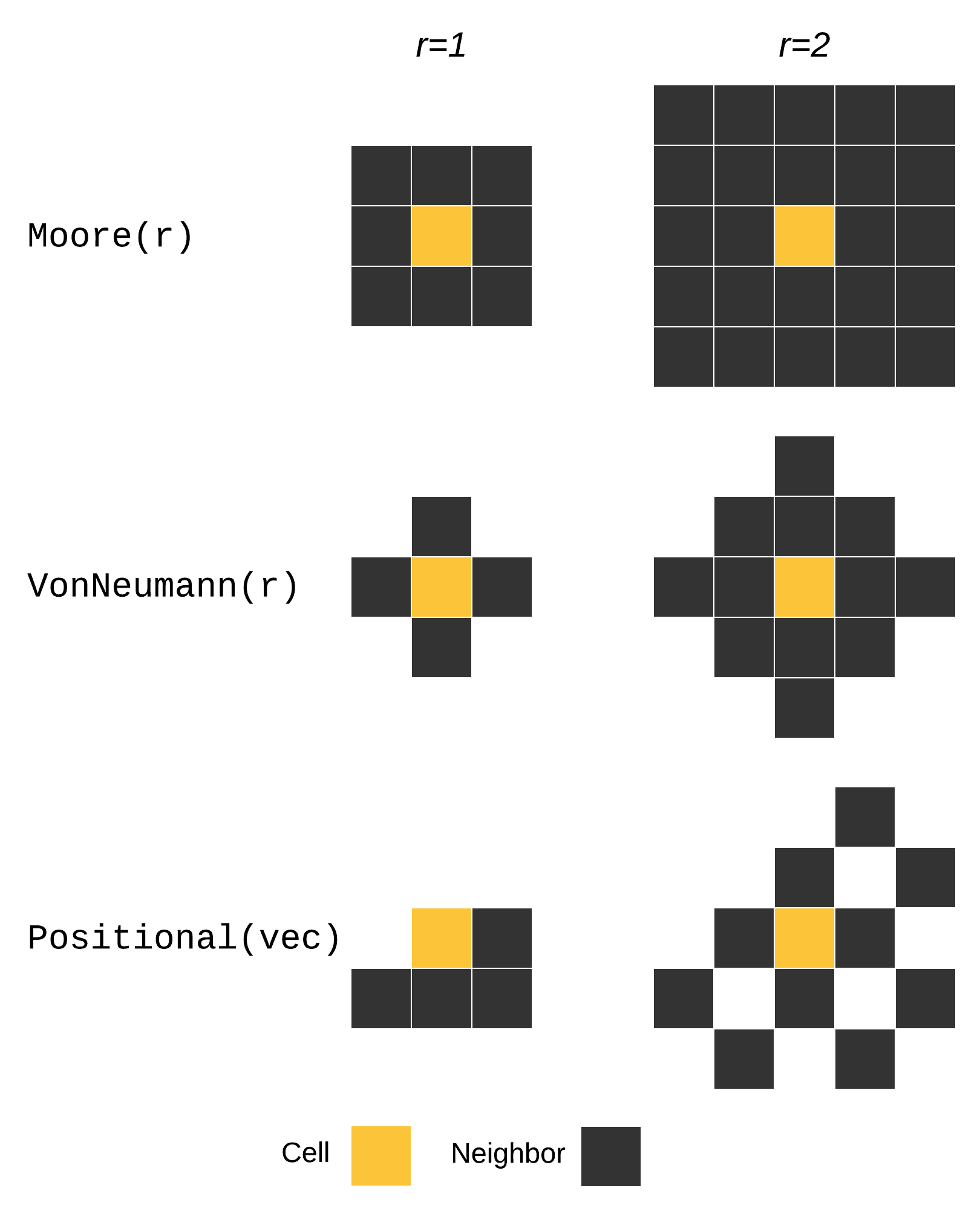
Neighborhoods can be used in NeighborhoodRule and SetNeighborhoodRule - the same shapes with different purposes. In a NeighborhoodRule the neighborhood specifies which cells around the current cell are returned as an iterable from the neighbors function. These can be counted, summed, compared, or multiplied with a kernel in an AbstractKernelNeighborhood, using kernelproduct.
In SetNeighborhoodRule neighborhoods give the locations of cells around the central cell, as [offsets] and absolute positions around the index of each neighbor. These can then be written to manually.
DynamicGrids.Neighborhoods.Moore — TypeMoore <: Neighborhood
Moore(radius::Int=1; ndims=2)
Moore(; radius=1, ndims=2)
Moore{R}(; ndims=2)
Moore{R,N}()Moore neighborhoods define the neighborhood as all cells within a horizontal or vertical distance of the central cell. The central cell is omitted.
Radius R = 1:
N = 1   N = 2

 ▄ ▄     █▀█
         ▀▀▀
Radius R = 2:
N = 1   N = 2

        █████
▀▀ ▀▀   ██▄██
        ▀▀▀▀▀
Using R and N type parameters removes runtime cost of generating the neighborhood, compated to passing arguments/keywords.
DynamicGrids.Neighborhoods.VonNeumann — TypeVonNeumann(radius=1; ndims=2) -> Positional
VonNeumann(; radius=1, ndims=2) -> Positional
VonNeumann{R,N}() -> PositionalA Von Neuman neighborhood is a damond-shaped, omitting the central cell:
Radius R = 1:
N = 1   N = 2

 ▄ ▄     ▄▀▄
          ▀
Radius R = 2:
N = 1   N = 2

         ▄█▄
▀▀ ▀▀   ▀█▄█▀
          ▀
In 1 dimension it is identical to Moore.
Using R and N type parameters removes runtime cost of generating the neighborhood, compated to passing arguments/keywords.
DynamicGrids.Neighborhoods.Window — TypeWindow <: Neighborhood
Window(; radius=1, ndims=2)
Window{R}(; ndims=2)
Window{R,N}()A neighboorhood of radius R that includes the central cell.
Radius R = 1:
N = 1   N = 2

 ▄▄▄     ███
         ▀▀▀
Radius R = 2:
N = 1   N = 2

        █████
▀▀▀▀▀   █████
▀▀▀▀▀DynamicGrids.Neighborhoods.AbstractPositionalNeighborhood — TypeAbstractPositionalNeighborhood <: NeighborhoodPositional neighborhoods are tuples of coordinates that are specified in relation to the central point of the current cell. They can be any arbitrary shape or size, but should be listed in column-major order for performance.
DynamicGrids.Neighborhoods.Positional — TypePositional <: AbstractPositionalNeighborhood
Positional(coord::Tuple{Vararg{Int}}...)
Positional(offsets::Tuple{Tuple{Vararg{Int}}})
Positional{O}()Neighborhoods that can take arbitrary shapes by specifying each coordinate, as Tuple{Int,Int} of the row/column distance (positive and negative) from the central point.
The neighborhood radius is calculated from the most distant coordinate. For simplicity the window read from the main grid is a square with sides 2r + 1 around the central point.
The dimensionality N of the neighborhood is taken from the length of the first coordinate, e.g. 1, 2 or 3.
Example radius R = 1:
N = 1   N = 2

 ▄▄      ▀▄
          ▀
Example radius R = 2:
N = 1   N = 2

         ▄▄
 ▀ ▀▀   ▀███
           ▀
Using the O parameter e.g. Positional{((1, 2), (1, 1))}() removes any runtime cost of generating the neighborhood.
DynamicGrids.Neighborhoods.LayeredPositional — TypeLayeredPositional <: AbstractPositional
LayeredPositional(layers::Positional...)Sets of Positional neighborhoods that can have separate rules for each set.
neighbors for LayeredPositional returns a tuple of iterators for each neighborhood layer.
Methods for use with neighborhood rules and neighborhoods
DynamicGrids.Neighborhoods.neighborhood — Functionneighborhood(x) -> NeighborhoodReturns a neighborhood object.
DynamicGrids.Neighborhoods.radius — Functionradius(rule, [key]) -> IntReturn the radius of a rule or ruleset if it has one, otherwise zero.
DynamicGrids.Neighborhoods.distances — Functiondistances(hood::Neighborhood)Get the center-to-center distance of each neighborhood position from the central cell, so that horizontally or vertically adjacent cells have a distance of 1.0, and a diagonally adjacent cell has a distance of sqrt(2.0).
Vales are calculated at compile time, so distances can be used inside rules with little overhead.
Useful with NeighborhoodRule:
DynamicGrids.Neighborhoods.neighbors — Functionneighbors(x::Union{Neighborhood,NeighborhoodRule}}) -> iterableReturns an indexable iterator for all cells in the neighborhood, either a Tuple of values or a range.
Custom Neighborhoods must define this method.
Useful with SetNeighborhoodRule:
DynamicGrids.Neighborhoods.positions — Functionpositions(x::Union{Neighborhood,NeighborhoodRule}}, cellindex::Tuple) -> iterableReturns an indexable iterable, over all cells as Tuples of each index in the main array. Useful in SetNeighborhoodRule for setting neighborhood values, or for getting values in an Aux array.
DynamicGrids.Neighborhoods.offsets — Functionoffsets(x) -> iterableReturns an indexable iterable over all cells, containing Tuples of the index offset from the central cell.
Custom Neighborhoods must define this method.
Convolution kernel neighborhoods
DynamicGrids.Neighborhoods.AbstractKernelNeighborhood — TypeAbstractKernelNeighborhood <: NeighborhoodAbstract supertype for kernel neighborhoods.
These can wrap any other neighborhood object, and include a kernel of the same length and positions as the neighborhood.
DynamicGrids.Neighborhoods.Kernel — TypeKernel <: AbstractKernelNeighborhood
Kernel(neighborhood, kernel)Wrap any other neighborhood object, and includes a kernel of the same length and positions as the neighborhood.
DynamicGrids.Neighborhoods.kernel — Functionkernel(hood::AbstractKernelNeighborhood) => iterableReturns the kernel object, an array or iterable matching the length of the neighborhood.
DynamicGrids.Neighborhoods.kernelproduct — Functionkernelproduct(rule::NeighborhoodRule})
kernelproduct(hood::AbstractKernelNeighborhood)
kernelproduct(hood::Neighborhood, kernel)Returns the vector dot product of the neighborhood and the kernel, although differing from dot in that the dot product is not take for vector members of the neighborhood - they are treated as scalars.
Low level use of neighborhoods
DynamicGrids.Neighborhoods.readwindow — Functionunsafe_readwindow(hood::Neighborhood, A::AbstractArray, I) => SArrayGet a single window square from an array, as an SArray, checking bounds.
DynamicGrids.Neighborhoods.unsafe_readwindow — Functionunsafe_readwindow(hood::Neighborhood, A::AbstractArray, I) => SArrayGet a single window square from an array, as an SArray, without checking bounds.
DynamicGrids.Neighborhoods.updatewindow — Functionupdatewindow(x, A::AbstractArray, I...) => NeighborhoodSet the window of a neighborhood to values from the array A around index I.
Bounds checks will reduce performance, aim to use unsafe_setwindow directly.
DynamicGrids.Neighborhoods.unsafe_updatewindow — Functionunsafe_setwindow(x, A::AbstractArray, I...) => NeighborhoodSet the window of a neighborhood to values from the array A around index I.
No bounds checks occur, ensure that A has padding of at least the neighborhood radius.
DynamicGrids.Neighborhoods.pad_axes — Functionpad_axes(A, hood::Neighborhood{R})
pad_axes(A, radius::Int)Add padding to axes.
DynamicGrids.Neighborhoods.unpad_axes — Functionunpad_axes(A, hood::Neighborhood{R})
unpad_axes(A, radius::Int)Remove padding from axes.
Generic neighborhood applicators
These can be used without the full simulation mechanisms, like broadcast.
DynamicGrids.Neighborhoods.broadcast_neighborhood — Functionbroadcast_neighborhood(f, hood::Neighborhood, As...)Simple neighborhood application, where f is passed each neighborhood in A, returning a new array.
The result is smaller than A on all sides, by the neighborhood radius.
DynamicGrids.Neighborhoods.broadcast_neighborhood! — Functionbroadcast_neighborhood!(f, hood::Neighborhood{R}, dest, sources...)Simple neighborhood broadcast where f is passed each neighborhood of src (except padding), writing the result of f to dest.
dest must either be smaller than src by the neighborhood radius on all sides, or be the same size, in which case it is assumed to also be padded.
Atomic methods for SetCellRule and SetNeighborhoodRule
Using these methods to modify grid values ensures cell independence, and also prevent race conditions with ThreadedCPU or [CuGPU].
DynamicGrids.add! — Functionadd!(data::WritableGridData, x, I...)Add the value x to a grid cell.
Example useage
using DynamicGrids
rule = SetCell{:a}() do data, a, cellindex
    dest, is_inbounds = inbounds(data, (jump .+ cellindex)...)

    # Update spotted cell if it's on the grid
    is_inbounds && add!(data[:a], state, dest...)
end

# output
SetCell{:a,:a}(
    f = var"#1#2"
)DynamicGrids.sub! — Functionsub!(data::WritableGridData, x, I...)Subtract the value x from a grid cell. See add! for example usage.
DynamicGrids.min! — Functionmin!(data::WritableGridData, x, I...)Set a gride cell to the minimum of x and the current value. See add! for example usage.
DynamicGrids.max! — Functionmax!(data::WritableGridData, x, I...)Set a gride cell to the maximum of x and the current value. See add! for example usage.
DynamicGrids.and! — Functionand!(data::WritableGridData, x, I...)
and!(A::AbstractArray, x, I...)Set the grid cell c to c & x. See add! for example usage.
DynamicGrids.or! — Functionor!(data::WritableGridData, x, I...)
or!(A::AbstractArray, x, I...)Set the grid cell c to c | x. See add! for example usage.
DynamicGrids.xor! — Functionxor!(data::WritableGridData, x, I...)
xor!(A::AbstractArray, x, I...)Set the grid cell c to xor(c, x). See add! for example usage.
Output
Output Types and Constructors
DynamicGrids.Output — TypeOutputAbstract supertype for simulation outputs.
Outputs are store or display simulation results, usually as a vector of grids, one for each timestep - but they may also sum, combine or otherwise manipulate the simulation grids to improve performance, reduce memory overheads or similar.
Simulation outputs are decoupled from simulation behaviour, and in many cases can be used interchangeably.
DynamicGrids.ArrayOutput — TypeArrayOutput <: Output
ArrayOutput(init; tspan::AbstractRange, [aux, mask, padval])A simple output that stores each step of the simulation in a vector of arrays.
Arguments
init: initialisationAbstractArrayArrayorNamedTupleofAbstractArrayArray.
Keywords (passed to Extent)
init: initialisationArray/NamedTuplefor grid/s.mask:BitArrayfor defining cells that will/will not be run.aux: NamedTuple of arbitrary input data. Useaux(data, Aux(:key))to access from aRulein a type-stable way.padval: padding value for grids with neighborhood rules. The default iszero(eltype(init)).tspan: Time span range. Never type-stable, only access this inmodifyrulemethods
An Extent object can be also passed to the extent keyword, and other keywords will be ignored.
DynamicGrids.ResultOutput — TypeResultOutput <: Output
ResultOutput(init; tspan::AbstractRange, kw...)A simple output that only stores the final result, not intermediate frames.
Arguments
init: initialisationArrayorNamedTupleofArray
Keywords (passed to Extent)
init: initialisationArray/NamedTuplefor grid/s.mask:BitArrayfor defining cells that will/will not be run.aux: NamedTuple of arbitrary input data. Useaux(data, Aux(:key))to access from aRulein a type-stable way.padval: padding value for grids with neighborhood rules. The default iszero(eltype(init)).tspan: Time span range. Never type-stable, only access this inmodifyrulemethods
An Extent object can be also passed to the extent keyword, and other keywords will be ignored.
DynamicGrids.TransformedOutput — TypeTransformedOutput(f, init; tspan::AbstractRange, kw...)An output that stores the result of some function f of the grid/s.
Arguments
f: a function or functor that accepts anAbstractArrayorNamedTupleofAbstractArraywith names matchinginit. TheAbstractArraywill be a view into the grid the same size as the init grids, removing any padding that has been added.init: initialisationArrayorNamedTupleofArray
Keywords
tspan:AbstractRangetimespan for the simulationaux: NamedTuple of arbitrary input data. Useget(data, Aux(:key), I...)to access from aRulein a type-stable way.mask:BitArrayfor defining cells that will/will not be run.padval: padding value for grids with neighborhood rules. The default iszero(eltype(init)).
WARNING: This feature is experimental. It may change in future versions, and may not be 100% reliable in all cases. Please file github issues if problems occur.
DynamicGrids.GraphicOutput — TypeGraphicOutput <: OutputAbstract supertype for Outputs that display the simulation frames.
All GraphicOutputs must have a GraphicConfig object and define a showframe method.
See REPLOutput for an example.
User Arguments for all GraphicOutput:
init: initialisationAbstractArrayorNamedTupleofAbstractArray
Minimum user keywords for all GraphicOutput:
Extent keywords:
init: initialisationArray/NamedTuplefor grid/s.mask:BitArrayfor defining cells that will/will not be run.aux: NamedTuple of arbitrary input data. Useaux(data, Aux(:key))to access from aRulein a type-stable way.padval: padding value for grids with neighborhood rules. The default iszero(eltype(init)).tspan: Time span range. Never type-stable, only access this inmodifyrulemethods
An Extent object can be also passed to the extent keyword, and other keywords will be ignored.
GraphicConfig keywords:
fps::Real: Frames per second.store::Bool: Whether to store frames likeArrayOutputor to disgard them after visualising. Very long simulation runs may fill available memory whenstore=true.
A GraphicConfig object can be also passed to the graphicconfig keyword, and other keywords will be ignored.
Internal keywords for constructors of objects extending GraphicOutput:
The default constructor will generate these objects and pass them to the inheriting object constructor, which must accept the following keywords:
frames: aVectorof simulation frames (NamedTupleorArray).running: ABool.extentanExtentobject.graphicconfigaGraphicConfigobject.
Users can also pass in these entire objects if required.
DynamicGrids.REPLOutput — TypeREPLOutput <: GraphicOutput
REPLOutput(init; tspan, kw...)An output that is displayed directly in the REPL. It can either store or discard simulation frames.
Arguments:
init: initialisationAbstractArrayArrayorNamedTupleofAbstractArrayArray.
Keywords
color: a color from Crayons.jlcutoff:Realcutoff point to display a full or empty cell. Default is0.5style:CharStyleBlock()orBraile()printing.Braileuses 1/4 the screen space ofBlock.
Extent keywords:
init: initialisationArray/NamedTuplefor grid/s.mask:BitArrayfor defining cells that will/will not be run.aux: NamedTuple of arbitrary input data. Useaux(data, Aux(:key))to access from aRulein a type-stable way.padval: padding value for grids with neighborhood rules. The default iszero(eltype(init)).tspan: Time span range. Never type-stable, only access this inmodifyrulemethods
An Extent object can be also passed to the extent keyword, and other keywords will be ignored.
GraphicConfig keywords:
fps::Real: Frames per second.store::Bool: Whether to store frames likeArrayOutputor to disgard them after visualising. Very long simulation runs may fill available memory whenstore=true.
A GraphicConfig object can be also passed to the graphicconfig keyword, and other keywords will be ignored.
e GraphicConfig object can be also passed to the graphicconfig keyword, and other keywords will be ignored.
DynamicGrids.ImageOutput — TypeImageOutput <: GraphicOutputAbstract supertype for Graphic outputs that display the simulation frames as RGB images.
ImageOutputs must have Extent, GraphicConfig and ImageConfig components, and define a showimage method.
See GifOutput for an example.
Although the majority of the code is maintained here to enable sharing and reuse, most ImageOutputs are not provided in DynamicGrids.jl to avoid heavy dependencies on graphics libraries. See DynamicGridsGtk.jl and DynamicGridsInteract.jl for implementations.
User Arguments for all GraphicOutput:
init: initialisationAbstractArrayorNamedTupleofAbstractArray
Minimum user keywords for all ImageOutput:
Extent keywords:
init: initialisationArray/NamedTuplefor grid/s.mask:BitArrayfor defining cells that will/will not be run.aux: NamedTuple of arbitrary input data. Useaux(data, Aux(:key))to access from aRulein a type-stable way.padval: padding value for grids with neighborhood rules. The default iszero(eltype(init)).tspan: Time span range. Never type-stable, only access this inmodifyrulemethods
An Extent object can be also passed to the extent keyword, and other keywords will be ignored.
GraphicConfig keywords:
fps::Real: Frames per second.store::Bool: Whether to store frames likeArrayOutputor to disgard them after visualising. Very long simulation runs may fill available memory whenstore=true.
A GraphicConfig object can be also passed to the graphicconfig keyword, and other keywords will be ignored.
ImageConfig keywords:
minval: Minimum value in the grid(s) to normalise for conversion to an RGB pixel. AVector/Matrixfor multiple grids, matching thelayoutarray. Note: The default is0, and will not be updated automatically for the simulation.maxval: Maximum value in the grid(s) to normalise for conversion to an RGB pixel. AVector/Matrixfor multiple grids, matching thelayoutarray. Note: The default is1, and will not be updated automatically for the simulation.font:Stringname of font to search for. A default will be guessed.text:TextConfig()ornothingfor no text. Default isTextConfig(; font=font).scheme: a ColorSchemes.jl colorscheme,ObjectSchemeor object that definesBase.get(obj, val)and returns aColoror a value that can be converted toColorusingARGB32(val).zerocolor: aColto use when values are zero, ornothingto ignore.maskcolor: aColorto use when cells are masked, ornothingto ignore.renderer:RendererlikeImageorLayout. Will be detected automatically, and usescheme,zerocolorandmaskcolorkeywords if available. Can be aVector/Matrixfor multiple grids, matching thelayoutarray.
An ImageConfig object can be also passed to the imageconfig keyword, and other keywords will be ignored.
Internal keywords for constructors of objects extending GraphicOutput:
The default constructor will generate these objects and pass them to the inheriting object constructor, which must accept the following keywords:
frames: aVectorof simulation frames (NamedTupleorArray).running: ABool.extentanExtentobject.graphicconfigaGraphicConfigobject.imageconfigaImageConfigobject.
Users can also pass in these entire objects if required.
DynamicGrids.GifOutput — TypeGifOutput <: ImageOutput
GifOutput(init; filename, tspan, kw...)Output that stores the simulation as images and saves a Gif file on completion.
Arguments:
init: initialisationAbstractArrayArrayorNamedTupleofAbstractArrayArray.
Keywords
Storing the gif:
filename: File path to save the gif file to.
Extent keywords:
init: initialisationArray/NamedTuplefor grid/s.mask:BitArrayfor defining cells that will/will not be run.aux: NamedTuple of arbitrary input data. Useaux(data, Aux(:key))to access from aRulein a type-stable way.padval: padding value for grids with neighborhood rules. The default iszero(eltype(init)).tspan: Time span range. Never type-stable, only access this inmodifyrulemethods
An Extent object can be also passed to the extent keyword, and other keywords will be ignored.
GraphicConfig keywords:
fps::Real: Frames per second.store::Bool: Whether to store frames likeArrayOutputor to disgard them after visualising. Very long simulation runs may fill available memory whenstore=true.
A GraphicConfig object can be also passed to the graphicconfig keyword, and other keywords will be ignored.
ImageConfig keywords:
minval: Minimum value in the grid(s) to normalise for conversion to an RGB pixel. AVector/Matrixfor multiple grids, matching thelayoutarray. Note: The default is0, and will not be updated automatically for the simulation.maxval: Maximum value in the grid(s) to normalise for conversion to an RGB pixel. AVector/Matrixfor multiple grids, matching thelayoutarray. Note: The default is1, and will not be updated automatically for the simulation.font:Stringname of font to search for. A default will be guessed.text:TextConfig()ornothingfor no text. Default isTextConfig(; font=font).scheme: a ColorSchemes.jl colorscheme,ObjectSchemeor object that definesBase.get(obj, val)and returns aColoror a value that can be converted toColorusingARGB32(val).zerocolor: aColto use when values are zero, ornothingto ignore.maskcolor: aColorto use when cells are masked, ornothingto ignore.renderer:RendererlikeImageorLayout. Will be detected automatically, and usescheme,zerocolorandmaskcolorkeywords if available. Can be aVector/Matrixfor multiple grids, matching thelayoutarray.
An ImageConfig object can be also passed to the imageconfig keyword, and other keywords will be ignored.
Renderers
DynamicGrids.Renderer — TypeRendererAbstract supertype for objects that convert a frame of the simulation into an ARGB32 image for display. Frames may be a single grid or a NamedTuple of multiple grids.
DynamicGrids.SingleGridRenderer — TypeSingleGridRenderer <: RendererAbstract supertype for Renderers that convert a single grid into an image array.
The first grid will be displayed if a SingleGridRenderer is used with a NamedTuple of grids.
DynamicGrids.Image — TypeImage <: SingleGridRenderer
Image(f=identity; scheme=ObjectScheme(), zerocolor=nothing, maskcolor=nothing)Converts output grids to a colorsheme.
Arguments
f: a function to convert value from the grid toRealoranRGB.Realwill be scaled by minval/maxval and be colored by thescheme.RGBis used directly in the output. This is useful for grids of complex objects, but not necessary for numbers. The default isidentity.
Keywords
scheme: a ColorSchemes.jl colorscheme,ObjectSchemeor object that definesBase.get(obj, val)and returns aColoror a value that can be converted toColorusingARGB32(val).zerocolor: aColto use when values are zero, ornothingto ignore.maskcolor: aColorto use when cells are masked, ornothingto ignore.
DynamicGrids.MultiGridRenderer — TypeMultiGridRenderer <: RendererAbstract type for Renderers that convert a frame containing multiple grids into a single image.
DynamicGrids.Layout — TypeLayout <: MultiGridRenderer
Layout(layout::Array, renderer::Matrix)Layout allows displaying multiple grids in a block layout, by specifying a layout matrix and a list of Images to be run for each.
Arguments
layout: AVectororMatrixcontaining the keys or numbers of grids in the locations to display them.nothing,missingor0values will be skipped.renderers:Vector/MatrixofImage, matching thelayout. Can benothingor any other value for grids not in layout.
DynamicGrids.SparseOptInspector — TypeSparseOptInspector()A Renderer that checks SparseOpt visually. Cells that do not run show in gray. Errors show in red, but if they do there's a bug.
Color schemes
Schemes from Colorschemes.jl can be used for the scheme argument to ImageOutput, Renderers. Greyscale control over the band of grey used, and is very fast. ObjectScheme is the default.
DynamicGrids.ObjectScheme — TypeObjectScheme
ObjectScheme()Default colorscheme. Similar to GreyScale for Number.
Other grid objects can define a custom method to return colors from composite objects:
DynamicGrids.to_rgb(::ObjectScheme, obj::MyObjectType) = ...Which must return an ARGB32 value.
DynamicGrids.Greyscale — TypeGreyscale
Greyscale(min=nothing, max=nothing)A greeyscale scheme ith better performance than using a Colorschemes.jl scheme as there is not array access or interpolation.
min and max are values between 0.0 and 1.0 that define the range of greys used.
Text labels
DynamicGrids.TextConfig — TypeTextConfig
TextConfig(; kw...)
TextConfig(face, namepixels, namepos, timepixels, timepos, fcolor, bcolor)Text configuration for printing timestep and grid name on the image.
Arguments / Keywords
font: AFreeTypeAbstraction.FTFont, or aStringwith the font name to look for. TheFTFontmay load more quickly.namepixelsandtimepixels: the pixel size of the font.timeposandnamepos: tuples that set the label positions, inIntpixels.fcolorandbcolor: the foreground and background colors, asARGB32.
Saving gifs
DynamicGrids.savegif — Functionsavegif(filename::String, o::Output; kw...)Write the output array to a gif.
Arguments
filename: File path to save the gif file to.output: AnOutputobject. Note that to make a gif, the output should stores frames, and run withstore=true, and@assert DynamicGrids.istored(o)should pass.
Keywords
ImageConfig keywords:
minval: Minimum value in the grid(s) to normalise for conversion to an RGB pixel. AVector/Matrixfor multiple grids, matching thelayoutarray. Note: The default is0, and will not be updated automatically for the simulation.maxval: Maximum value in the grid(s) to normalise for conversion to an RGB pixel. AVector/Matrixfor multiple grids, matching thelayoutarray. Note: The default is1, and will not be updated automatically for the simulation.font:Stringname of font to search for. A default will be guessed.text:TextConfig()ornothingfor no text. Default isTextConfig(; font=font).scheme: a ColorSchemes.jl colorscheme,ObjectSchemeor object that definesBase.get(obj, val)and returns aColoror a value that can be converted toColorusingARGB32(val).zerocolor: aColto use when values are zero, ornothingto ignore.maskcolor: aColorto use when cells are masked, ornothingto ignore.renderer:RendererlikeImageorLayout. Will be detected automatically, and usescheme,zerocolorandmaskcolorkeywords if available. Can be aVector/Matrixfor multiple grids, matching thelayoutarray.
Output interface
These are used for defining your own outputs and GridProcessors, not for general scripting.
DynamicGrids.AbstractExtent — TypeAbstractExtentAbstract supertype for Extent objects, that hold all variables related to space and time in a simulation. Usually the field of an output.
DynamicGrids.Extent — TypeExtent <: AbstractExtent
Extent(init, mask, aux, padval, tspan)
Extent(; init, tspan, mask=nothing, aux=nothing, padval=zero(eltype(init)), kw...)Container for extensive variables: spatial and timeseries data. These are kept separate from rules to allow application of rules to alternate spatial and temporal contexts.
Extent is not usually constructed directly by users, but it can be passed to Output constructors instead of init, mask, aux and tspan.
Arguments/Keywords
init: initialisationArray/NamedTuplefor grid/s.mask:BitArrayfor defining cells that will/will not be run.aux: NamedTuple of arbitrary input data. Useaux(data, Aux(:key))to access from aRulein a type-stable way.padval: padding value for grids with neighborhood rules. The default iszero(eltype(init)).tspan: Time span range. Never type-stable, only access this inmodifyrulemethods
DynamicGrids.extent — FunctionDynamicGrids.isasync — Functionisasync(o::Output) => BoolOutput interface method.
Check if the output should run asynchonously. Default is false.
DynamicGrids.storeframe! — Functionstoreframe!(o::Output, data::AbstractSimData)Store the current simulaiton frame in the output.
DynamicGrids.isrunning — Functionisrunning(o::Output) => BoolOutput interface method.
Check if the output is running. Prevents multiple versions of sim! running on the same output for asynchronous outputs.
DynamicGrids.isshowable — Functionisshowable(o::Output, f::Int) => BoolOutput interface method.
Check if the output can be shown visually, where f is the frame number. Default is false.
DynamicGrids.isstored — Functionisastored(o::Output) => BoolOutput interface method.
Check if the output is storing each frame, or just the the current one. Default is true.
DynamicGrids.initialise! — FunctionDynamicGrids.finalise! — Functionfinalise!(o::Output, data::AbstractSimData)Output interface method.
Finalise the output at the end of the simulation.
DynamicGrids.frameindex — Functionframeindex(o::Output, data::AbstractSimData)Output interface method.
Get the index of the current frame in the output. Every frame has an index of 1 if the simulation isn't stored.
GraphicOutput interface
Also includes Output interface.
DynamicGrids.GraphicConfig — TypeGraphicConfig
GraphicConfig(; fps=25.0, store=false)Config and variables for graphic outputs.
Keywords
fps::Real: Frames per second.store::Bool: Whether to store frames likeArrayOutputor to disgard them after visualising. Very long simulation runs may fill available memory whenstore=true.
DynamicGrids.graphicconfig — Functiongraphicconfig(output::GraphicOutput) => GraphicConfigGraphicOutput interface method. Return an GraphicConfig object.
DynamicGrids.fps — Functionfps(o::Output) => RealGraphicOutput interface method.
Get the frames per second the output will run at. The default is nothing - the simulation runs at full speed.
DynamicGrids.setfps! — Functionsetfps!(o::Output, x)GraphicOutput interface method.
Set the frames per second the output will run at.
DynamicGrids.showframe — Functionshowframe(o::Output, data::AbstractSimData)
showframe(frame::NamedTuple, o::Output, data::AbstractSimData)
showframe(frame::AbstractArray, o::Output, data::AbstractSimData)GraphicOutput interface method.
Display the grid/s somehow in the output, if it can do that.
DynamicGrids.initialisegraphics — Functioninitalisegraphics(o::Output, data::AbstractSimData)GraphicOutput interface method.
Initialise the output graphics at the start of the simulation, if it has graphics.
DynamicGrids.finalisegraphics — Functionfinalisegraphics(o::Output, data::AbstractSimData)GraphicOutput interface method.
Finalise the output graphics at the end of the simulation, if it has graphics.
ImageOutput components and interface
Also uses Output and GraphicOutput interfaces.
DynamicGrids.ImageConfig — TypeImageConfig
ImageConfig(init; kw...)Common configuration component for all ImageOutput.
Arguments
initoutput init object, used to generate other arguments automatically.
Keywords
minval: Minimum value in the grid(s) to normalise for conversion to an RGB pixel. AVector/Matrixfor multiple grids, matching thelayoutarray. Note: The default is0, and will not be updated automatically for the simulation.maxval: Maximum value in the grid(s) to normalise for conversion to an RGB pixel. AVector/Matrixfor multiple grids, matching thelayoutarray. Note: The default is1, and will not be updated automatically for the simulation.font:Stringname of font to search for. A default will be guessed.text:TextConfig()ornothingfor no text. Default isTextConfig(; font=font).scheme: a ColorSchemes.jl colorscheme,ObjectSchemeor object that definesBase.get(obj, val)and returns aColoror a value that can be converted toColorusingARGB32(val).zerocolor: aColto use when values are zero, ornothingto ignore.maskcolor: aColorto use when cells are masked, ornothingto ignore.renderer:RendererlikeImageorLayout. Will be detected automatically, and usescheme,zerocolorandmaskcolorkeywords if available. Can be aVector/Matrixfor multiple grids, matching thelayoutarray.
DynamicGrids.imageconfig — Functionimageconfig(output::ImageOutput) => ImageConfigImageOutpu interface method. Return an ImageConfig object.
DynamicGrids.showimage — Functionshowimage(image::AbstractArray, o::ImageOutput)
showimage(image::AbstractArray, o::ImageOutput, data::AbstractSimData)ImageOutput interface method.
Display an image generated from the grid, a required method for all ImageOutput.
DynamicGrids.render! — Functionrender!(o::ImageOutput, data::AbstractSimData)
render!(imbuf, renderer::Renderer, o::ImageOutput, data::AbstractSimData, grids)Convert a grid or NamedRuple of grids to an ARGB32 image, using an Renderer.
Rendered pixels are written to the image buffer matrix.
DynamicGrids.to_rgb — Functionto_rgb(val) => ARGB32
to_rgb(scheme, val) => ARGB32ImageOutput interface method.
Display an image generated from the grid, a required method for all ImageOutput.
Custom grid object will need to add methods for converting the object to a color,
to_rgb(::ObjectScheme, obj::CustomObj) = ...`For use with other colorschemes, a method that calls get with a Real value obtained from the object will be required:
to_rgb(scheme, obj::CustomObj) = ARGB32(get(scheme, real_from_obj(obj)))Custom grid element types
It is common to use Bool, Int or Float64 as the contents of a grid. But a range of object types can be used if they meet the interface criteria.
Immutable, isbits objects are usually better and the only type officially to work - as they are loaded directly in the simulation. Mutable objects, especially containing pointers, may lead to incorrect stored results, and wont work at all on GPUs.
Methods to define are:
zero: define zero of the object typeoneunit: define one of the object typeisless: define comparison between two of the objects*: multiplication by aRealscalar./: division by aRealscalar.+: addition to another object of the same type-: subtraction from another object of the same typeto_rgb: return andARGB32to visualise the object as a pixel
In this example we define a struct with two fields. You will need to determine the correct behaviours for your own types, but hopefully this will get you started.
struct MYStruct{A,B}
    a::A
    b::B
end

Base.isless(a::MyStruct, b::MyStruct) = isless(a.a, b.a)
Base.zero(::Type{<:MyStruct{T1,T2}}) where {T1,T2} = MyStruct(zero(T1), zero(T2))
Base.oneunit(::Type{<:MyStruct{T1,T2}}) where {T1,T2} = MyStruct(one(T1), one(T2))

Base.:*(x::MyStruct, x::Number) = MyStruct(x.a * x, x.b * x)
Base.:*(x::Number, x::MyStruct) = MyStruct(x * x.a, x * x.b)
Base.:/(x::MyStruct, x::Number) = MyStruct(x.a / x, x.b / x)
Base.:+(x1::MyStruct, x2::MyStruct) = MyStruct(x1.a + x2.a, x1.b + x2.b)
Base.:-(x1::MyStruct, x2::MyStruct) = MyStruct(x1.a - x2.a, x1.b - x2.b)
To generate rgb colors for an ImageOuput, you must define to_rgb, at least for the default ObjectScheme, but this can also be done for other schemes such as ColorSchemes.jl, or GreyScale, by calling get on the scheme and a Real value. Note that the objects will be normalised to values between zero and one by minval and maxval scalars prior to this, using the division operators defined above. It is preferable to use minval and maxval over normalising in to_rgb - as this will not be as flexible for scripting.
DynamicGrids.to_rgb(::ObjectScheme, obj::MyStruct) = ARGB32(obj.a, obj.b, 0)
DynamicGrids.to_rgb(scheme, obj::MyStruct) = get(scheme, obj.a)
See the test/objectgrids.jl tests for more details on using complex objects in grids.